| attribute | description |
|---|---|
| Resource name | CEDEL2: Corpus Escrito del Español como L2. |
| Data source | http://cedel2.learnercorpora.com/, https://doi.org/10.1177/02676583211050522 |
| Data sampling frame | Corpus that contains samples of the language produced from learners of Spanish as a second language. For comparative purposes, it also contains a native control subcorpus of the language produced by native speakers of Spanish from different varieties (peninsular Spanish and all varieties of Latin American Spanish), so it can be used as a native corpus in its own right. |
| Data collection date(s) | 2006-2020. |
| Data format | CSV file. Each row corresponds to a writing sample. Each column is an attribute of the writing sample. |
| Data schema | A CSV file for L2 learners and a CSV file for native speakers. |
| License | CC BY-NC-ND 3.0 ES |
| Attribution | Lozano, C. (2022). CEDEL2: Design, compilation and web interface of an online corpus for L2 Spanish acquisition research. Second Language Research, 38(4), 965-983. https://doi.org/10.1177/02676583211050522. |
5 Acquire
As we start down the path to executing our research blueprint, our first step is to acquire the primary data that will be employed in the project. This chapter covers two commonly-used strategies for acquiring corpus data: downloads and APIs. We will encounter various file formats and folder structures in the process and we will address how to effectively organize our data for subsequent processing. Crucial to our efforts is the process of documenting our data. We will learn to provide data origin information to ensure key characteristics of the data and its source are documented. Along the way, we will explore R coding concepts including control statements and custom functions relevant to the task of acquiring data. By the end of this chapter, you will not only be adept at acquiring data from diverse sources but also capable of documenting it comprehensively, enabling you to replicate the process in the future.
5.1 Downloads
The most common and straightforward method for acquiring corpus data is through direct downloads. In a nutshell, this method involves navigating to a website, locating the data, and downloading it to your computing environment. In some cases access to the data requires manual intervention and in others the process can be implemented programmatically. The data may be contained in a single file or multiple files. The files may be archived or unarchived. The data may be hierarchically organized or not. Each resource will have its own unique characteristics that will influence the process of acquiring the data. In this section we will work through a few examples to demonstrate the general process of acquiring data through downloads.
Manual
In contrast to the other data acquisition methods we will cover in this chapter, manual downloads require human intervention. This means that manual downloads are non-reproducible in a strict sense and require that we keep track of and document our procedure. It is a very common for research projects to acquire data through manual downloads as many data resources require some legwork before they are accessible for downloading. These can be resources that require institutional or private licensing and fees, require authorization/ registration, and/ or are only accessible via resource search interfaces.
The resource we will use for this demonstration is the Corpus Escrito del Español como L2 (CEDEL2) (Lozano, 2009), a corpus of Spanish learner writing. It includes L2 writing from students with a variety of L1 backgrounds. For comparative puposes it also includes native writing for Spanish, English, and several other languages.
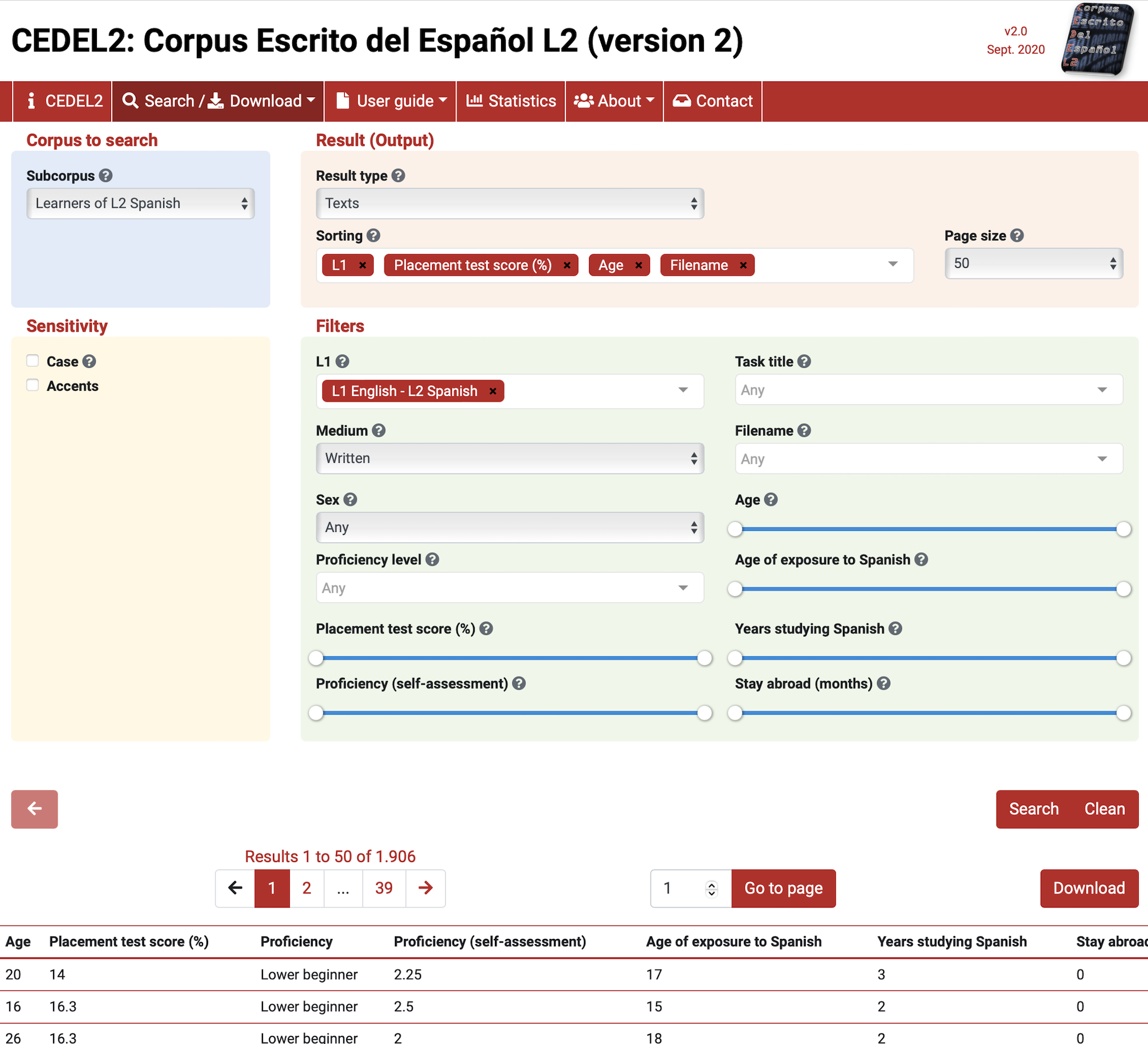
The CEDEL2 corpus is a freely available resource, but to access the data you must first use a search interface to select the relevant characteristics of the data of interest. Following the search/ download link you can find a search interface that allows the user to select the subcorpus and filter the results by a set of attributes.
For this example let’s assume that we want to acquire data to use in a study comparing the use of the Spanish preterite and imperfect past tense aspect in written texts by English L1 learners of Spanish to native Spanish speakers. To acquire data for such a project, we will first select the subcorpus “Learners of L2 Spanish”. We will set the results to provide full texts and filter the results to “L1 English - L2 Spanish”. Additionally, we will set the medium to “Written”. This will provide us with a set of texts for the L2 learners that we can use for our study. The search parameters and results are shown in Figure 5.1.
The ‘Download’ link now appears for this search criteria. Following this link will provide the user a form to fill out. This particular resource allows for access to different formats to download (Texts only, Texts with metadata, CSV (Excel), CSV (Others)). I will select the ‘CSV (Others)’ option so that the data is structured for easier processing downstream in subsequent processing steps. Then I save the CSV in the data/original/ directory of my project and create a sub-directory named cedel2/, as seen in Snippet 5.1.
Snippet 5.1 Project structure for the CEDEL2 corpus learner data download
data/
├── analysis/
├── derived/
└── original/
    └── cedel2/
    └── cedel2-l1-english-learners.csv
Note that the file is named cedel2-l1-english-learners.csv to reflect the search criteria used to acquire the data. In combination with other data documentation, this will help us to maintain transparency.
Now, after downloading the L2 learner and the native speaker data into the appropriate directory, we move on to the next processing step, right? Not so fast! Imagine we are working on a project with a collaborator. How will they know where the data came from? What if we need to come back to this data in the future? How will we know what characteristics we used to filter the data? The directory and filenames may not be enough. To address these questions we need to document the origin of the data, and in the case of data acquired through manual downloads, we need to document the procedures we took to acquire the data to the best of our ability.
As discussed in Section 2.3.1, all acquired data should be accompanied by a data origin file. The majority of this information can typically be identified on the resource’s website and/ or the resource’s documentation. In the case of the CEDEL2 corpus, the corpus homepage provides most of the information we need. The data origin file for the CEDEL2 corpus is seen in Table 5.1.
Structurally, data documentation files should be stored close to the data they describe. So for our data origin file this means adding it to the data/original/ directory. Naming the file in a transparent way is also important. I’ve named the file cedel2_do.csv to reflect the name of the corpus, the meaning of the file as data origin with a suffixed *_do, and the file extension .csv* to reflect the file format. CSV files reflect tabular content. It is not required that data origin files are tabular, but it makes it easier to read and display them in literate programming documents.
Given this is a manual download we also need to document the procedure used to retrieve the data in prose. The script in the process/ directory that is typically used to acquire the data is not used to programmatically retrieve data in this case. However, to keep things predictable we will use this file to document the download procedure. I’ve created a Quarto file named 1_acquire_data.qmd in the process/ directory of my project. A glimpse at the directory structure of the project at this point is seen in Snippet 5.2.
Even though the 1_acquire_data.qmd file is not used to programmatically retrieve the data, it is still a useful place to document the download procedure. This includes the URL of the resource, the search criteria used to filter the data, and the file format and location of the data. It is also good to include and display your data origin file in this file as a formatted table.
Snippet 5.2 Project structure for the CEDEL2 corpus data acquisition
project/
├── process/
│   ├── 1_acquire_data.qmd
│   └── ...
├── data/
│   ├── analysis/
│   ├── derived/
│   └── original/
│       ├── cedel2_do.csv
│       └── cedel2/
│           ├── cedel2-l1-english-learners.csv
│           └── cedel2-native-spanish-speakers.csv
├── reports/
├── DESCRIPTION
├── Makefile
└── README
Manually downloading other resources will inevitably include unique processes for obtaining the data, but in the end the data should be archived in the project structure in the data/original/ directory and documented in the appropriate places. Note that acquired data is always treated as ‘read-only’, meaning it is not modified in any way. This gives us a fixed starting point for subsequent steps in the data preparation process.
Programmatic
There are many resources that provide corpus data that is directly accessible for which programmatic downloads can be applied. A programmatic download is a download in which the process can be automated through code. Thus, this is a reproducible process. The data can be acquired by anyone with access to the necessary code.
In this case, and subsquent data acquisition procedures in this chapter, we use the 1_acquire_data.qmd Quarto file to its full potential intermingling prose, code, and code comments to execute and document the download procedure.
To illustrate how this works to conduct a programmatic download, we will work with the Switchboard Dialog Act Corpus (SWDA) (University of Colorado Boulder, 2008). The version that we will use is found on the Linguistic Data Consortium under the Switchboard-1 Release 2 Corpus. The corpus and related documentation are linked on the catalog page https://catalog.ldc.upenn.edu/docs/LDC97S62/.
From the documentation we learn that the corpus contains transcripts for 1155 5-minute two-way telephone conversations among English speakers for all areas of the United States. The speakers were given a topic to discuss and the conversations were recorded. The corpus metadata and annotations for sociolinguistic and discourse features.
This corpus, as you can image, could support a wide range of interesting reseach questions. Let’s assume we are following research conducted by Tottie (2011) to explore the use of filled pauses such as “um” and “uh” and traditional sociolinguistic variables such as sex, age, and education in spontaneous speech by American English speakers.
With this goal in mind, let’s get started writing the code to download and organize the data in our project directory. First, we need to identify the URL (Uniform Resource Locator) for the data that we want to download. More often than not this file will be some type of archive file with an extension such as .zip (Zipped file), .tar (Tarball file), or tar.gz (Gzipped tarball file), which is the case for the SWDA corpus. Archive files make downloading multiple files easy by grouping files and directories into one file.
In R, we can use the download.file() function from base R, as seen in Example 5.1. The download.file() function minimally requires two arguments: url and destfile. These correspond to the file to download and the location where it is to be saved to disk. To break out the process a bit, I will assign the URL and destination file path to variables and then use the download.file() function to download the file.
Example 5.1
# URL to SWDA corpus archive file
file_url <-
  "https://catalog.ldc.upenn.edu/docs/LDC97S62/swb1_dialogact_annot.tar.gz"

# Relative path to project/data/original directory
file_path <- "../data/original/swda.tar.gz"

# Download SWDA corpus archive file
download.file(url = file_url, destfile = file_path)As we can see looking at the directory structure, in Snippet 5.3, the swda.tar.zip file has been added to the data/original/ directory.
Snippet 5.3 Project structure for the SWDA archive file download
data/
├── analysis/
├── derived/
└── original/
    └── swda.tar.zip
Once an archive file is downloaded, however, the file needs to be ‘unarchived’ to reveal the directory structure and files. To unarchive this .tar.gz file we use the untar() function with the arguments tarfile pointing to the .tar.gz file and exdir specifying the directory where we want the files to be extracted to. Again, I will assign the arguments to variables. Then we can unarchive the file using the untar() function.
Example 5.2
The directory structure of data/ in Snippet 5.4 now shows the swda.tar.gz file and the swda directory that contains the unarchived directories and files.
Snippet 5.4 Project structure for the SWDA files unarchived
data/
├── analysis/
├── derived/
└── original/
    ├── swda/
    │   ├── README
    │   ├── doc/
    │   ├── sw00utt/
    │   ├── sw01utt/
    │   ├── sw02utt/
    │   ├── sw03utt/
    │   ├── sw04utt/
    │   ├── sw05utt/
    │   ├── sw06utt/
    │   ├── sw07utt/
    │   ├── sw08utt/
    │   ├── sw09utt/
    │   ├── sw10utt/
    │   ├── sw11utt/
    │   ├── sw12utt/
    │   └── sw13utt/
    └── swda.tar.gz
At this point we have acquired the data programmatically and with this code as part of our workflow anyone could run this code and reproduce the same results.
The code as it is, however, is not ideally efficient. First, the swda.tar.gz file is not strictly needed after we unarchive it and it occupies disk space, if we keep it. And second, each time we run this code the file will be downloaded from the remote server and overwrite the existing data. This leads to unnecessary data transfer and server traffic and will overwrite the data if it already exists in our project directory which could be problematic if the data changes on the remote server. Let’s tackle each of these issues in turn.
To avoid writing the swda.tar.gz file to disk (long-term) we can use the tempfile() function to open a temporary holding space for the file in the computing environment. This space can then be used to store the file, unarchive it, and then the temporary file will automatically be deleted. We assign the temporary space to an R object we will name temp_file with the tempfile() function. This object can now be used as the value of the argument destfile in the download.file() function.
Example 5.3
At this point our downloaded file is stored temporarily on disk and can be accessed and unarchived to our target directory using temp_file as the value for the argument tarfile from the untar() function. I’ve assigned our target directory path to extract_to_dir and used it as the value for the argument exdir.
Example 5.4
Our directory structure in Example 5.4 is the same as in Snippet 5.4, minus the swda.tar.gz file.
The second issue I raised concerns the fact that running this code as part of our project will repeat the download each time our script is run. Since we would like to be good citizens and avoid unnecessary traffic on the web and avoid potential issues in overwriting data, it would be nice if our code checked to see if we already have the data on disk and if it exists, then skip the download, if not then download it.
The desired functionality we’ve described can be implemented using the if() function. The if() function is one of a class of functions known as control statements. Control statments allow us to control the flow of our code by evaluating logical statements and processing subsequent code based on the logical value it is passed as an argument.
So in this case we want to evaluate whether the data directory exists on disk. If it does then skip the download, if not, proceed with the download. In combination with else which provides the ‘if not’ part of the statement, we have the following logical flow in Example 5.5.
We can simplify this statement by using the ! operator which negates the logical value of the statement it precedes. So if the directory exists, !DIRECTORY_EXISTS will return FALSE and if the directory does not exist, !DIRECTORY_EXISTS will return TRUE. In other words, if the directory does not exist, download the data. This is shown in Example 5.6.
Now, to determine if a directory exists in our project directory we will turn to {fs} (Hester, Wickham, & Csárdi, 2024). {fs} provides a set of functions for interacting with the file system, including dir_exists(). dir_exists() takes a path to a directory as an argument and returns the logical value, TRUE, if that directory exists, and FALSE if it does not.
We can use this function to evaluate whether the directory exists and then use the if() function to process the subsequent code based on the logical flow we set out in Example 5.6. Applied to our project, the code will look like Example 5.7.
Example 5.7
# Load the {fs} package
library(fs)

# URL to SWDA corpus archive file
file_url <-
  "https://catalog.ldc.upenn.edu/docs/LDC97S62/swb1_dialogact_annot.tar.gz"

# Create a temporary file space for our .tar.gz file
temp_file <- tempfile()

# Assign our target directory to `extract_to_dir`
extract_to_dir <- "../data/original/swda/"

# Check if our target directory exists
# If it does not exist, download the file and extract it
if (!dir_exists(extract_to_dir)) {
  # Download SWDA corpus archive file
  download.file(file_url, temp_file)

  # Unarchive/ decompress .tar.gz file and extract to our target directory
  untar(tarfile = temp_file, exdir = extract_to_dir)
}
The code in Example 5.7 is added to the 1_acquire_data.qmd file. When this file is run, the SWDA corpus data will be downloaded and extracted to our project directory. If the data already exists, the download will be skipped, just as we wanted.
Now, before we move on, we need to make sure to document the process. Now that our Quarto document includes code we can review, explain, and comment this process. And, as always, create a data origin file as with the relevant information. The data origin file will be stored in the data/original/ directory and the Quarto file will be stored in the process/ directory.
We’ve leveraged R to automate the download and extraction of the data, depending on the existence of the data in our project directory. But you may be asking yourself, “Can’t I just navigate to the corpus page and download the data manually myself?” The simple answer is, “Yes, you can.” The more nuanced answer is, “Yes, but consider the trade-offs.”
The following scenarios highlight the some advantages to automating the process. If you are acquiring data from multiple files, it can become tedious to document the manual process for each file such that it is reproducible. It’s possible, but it’s error prone.
Now, if you are collaborating with others, you will want to share this data with them. It is very common to find data that has limited restrictions for use in academic projects, but the most common limitation is redistribution. This means that you can use the data for your own research, but you cannot share it with others. If you plan on publishing your project to a code repository to share the data as part of your reproducible project, you would be violating the terms of use for the data. By including the programmatic download in your project, you can ensure that your collaborators can easily and effectively acquire the data themselves and that you are not violating the terms of use.
5.2 APIs
A convenient alternative method for acquiring data in R is through package interfaces to web services. These interfaces are built using R code to make connections with resources on the web through Application Programming Interfaces (APIs). Websites such as Project Gutenberg, Twitter, Reddit, and many others provide APIs to allow access to their data under certain conditions, some more limiting for data collection than others. Programmers (like you!) in the R community take up the task of wrapping calls to an API with R code to make accessing that data from R convenient, and of course reproducible.
In addition to popular public APIs, there are also APIs that provide access to repositories and databases which are of particular interest to linguists. For example, Wordbank provides access to a large collection of child language corpora through {wordbankr} (Braginsky, 2024), and Glottolog, World Atlas of Language Structures (WALS), and PHOIBLE provide access to large collections of language metadata that can be accessed through {lingtypology} (Moroz, 2017).
Let’s work with an R package that provides access to the TalkBank database. The TalkBank project (Macwhinney, 2024) contains a large collection of spoken language corpora from various contexts: conversation, child language, multilinguals, etc. Resource information, web interfaces, and links to download data in various formats can be found by perusing individual resources linked from the main page. However, {TBDBr} (Kowalski & Cavanaugh, 2024) provides convenient access to corpora using R once a corpus resource is identified.
The CABNC (Albert, de Ruiter, & de Ruiter, 2015) contains the demographically sampled portion of the spoken portion of the British National Corpus (BNC) (Leech, 1992).
Useful for a study aiming to research spoken British English, either in isoloation or in comparison to American English (SWDA).
First, we need to install and load {TBDBr}, as in Example 5.8.
{TBDBr} provides a set of common get*() functions for acquiring data from the TalkBank corpus resources. These include: getParticipants(), getTranscripts(), getTokens(), getTokenTypes(), and getUtterances().
For each of these function the first argument is corpusName, which is the name of the corpus resource as it appears in the TalkBank database. The second argument is corpora, which takes a character vector describing the path to the data. For the CABNC, these arguments are "ca" and c("ca", "CABNC") respectively. To determine these values, TBDBr provides the getLegalValues() interactive function which allows you to interactively select the repository name, corpus name, and transcript name, if necessary.
Another important aspect of these function is that they return data frame objects. Since we are accessing data that is in a structured database, this makes sense. However, we should always check the documentation for the object type that is returned by function to be aware of how to work with the data.
Let’s start by retrieving the utterance data for the CABNC and preview the data frame it returns using glimpse().
Example 5.9
# Set corpus_name and corpus_path
corpus_name <- "ca"
corpus_path <- c("ca", "CABNC")

# Get utterance data
utterances <-
  getUtterances(
    corpusName = corpus_name,
    corpora = corpus_path
    )

# Preview the data
glimpse(utterances)
Rows: 235,901
Columns: 10
$ filename <list> "KB0RE000", "KB0RE000", "KB0RE000", "KB0RE000", "KB0RE000",…
$ path <list> "ca/CABNC/KB0/KB0RE000", "ca/CABNC/KB0/KB0RE000", "ca/CABNC…
$ utt_num <list> 0, 1, 2, 3, 4, 5, 6, 7, 8, 9, 10, 11, 12, 13, 14, 15, 16, 1…
$ who <list> "PS002", "PS006", "PS002", "PS006", "PS002", "PS006", "PS00…
$ role <list> "Unidentified", "Unidentified", "Unidentified", "Unidentifi…
$ postcodes <list> <NULL>, <NULL>, <NULL>, <NULL>, <NULL>, <NULL>, <NULL>, <NU…
$ gems <list> <NULL>, <NULL>, <NULL>, <NULL>, <NULL>, <NULL>, <NULL>, <NU…
$ utterance <list> "You enjoyed yourself in America", "Eh", "did you", "Oh I c…
$ startTime <list> "0.208", "2.656", "2.896", "3.328", "5.088", "6.208", "8.32…
$ endTime <list> "2.672", "2.896", "3.328", "5.264", "6.016", "8.496", "9.31…Inspecting the output from Example 5.9, we see that the data frame contains 235,901 observations and 10 variables.
The summary provided by glimpse() also provides other useful information. First, we see the data type of each variable. Interestingly, the data type for each variable in the data frame is a list object. Being that a list is two-dimensional data type, like a data frame, we have two-dimensional data inside two-dimensional data. This is known as a nested structure. We will work with nested structures in more depth later, but for now it will suffice to say that we would like to ‘unnest’ these lists and reveal the list-contained vector types at the data frame level.
To do this we will pass the utterances data frame to the, appropriately named, unnest() function from {tidyr} (Wickham, Vaughan, & Girlich, 2024). unnest() takes a data frame and a vector of variable names to unnest, cols = c(). To unnest all variables, we will use the everything() function from {dplyr} to select all variables at once. We will use the result to overwrite the utterances object with the unnested data frame.
Example 5.10
# Unnest the data frame
utterances <-
  utterances |>
  unnest(cols = everything())

# Preview the data
glimpse(utterances)
Rows: 235,901
Columns: 10
$ filename <chr> "KB0RE000", "KB0RE000", "KB0RE000", "KB0RE000", "KB0RE000", …
$ path <chr> "ca/CABNC/KB0/KB0RE000", "ca/CABNC/KB0/KB0RE000", "ca/CABNC/…
$ utt_num <dbl> 0, 1, 2, 3, 4, 5, 6, 7, 8, 9, 10, 11, 12, 13, 14, 15, 16, 17…
$ who <chr> "PS002", "PS006", "PS002", "PS006", "PS002", "PS006", "PS002…
$ role <chr> "Unidentified", "Unidentified", "Unidentified", "Unidentifie…
$ postcodes <lgl> NA, NA, NA, NA, NA, NA, NA, NA, NA, NA, NA, NA, NA, NA, NA, …
$ gems <lgl> NA, NA, NA, NA, NA, NA, NA, NA, NA, NA, NA, NA, NA, NA, NA, …
$ utterance <chr> "You enjoyed yourself in America", "Eh", "did you", "Oh I co…
$ startTime <chr> "0.208", "2.656", "2.896", "3.328", "5.088", "6.208", "8.32"…
$ endTime <chr> "2.672", "2.896", "3.328", "5.264", "6.016", "8.496", "9.312…The output from Example 5.10 shows that the variables are now one-dimensional vector types.
Returning to the information about our data frame from glimpse(), the second thing to notice is we get a short preview of the values for each variable. There are a couple things we can gleen from this. One is that we can confirm or clarify the meaning of the variable names by looking at the values. The other thing to consider is whether the values show any patterns that may be worthy of more scrutiny. For example, various variables appear to contain the same values for each observation. For a variable like filename, this is expected as the first values likely correspond to the same file. However, for the variables postcodes and gems the values are ‘NA’. This suggests that these variables may not contain any useful information and we may want to remove them later.
For now, however, we want to acquire and store the data in its original form (or as closely as possible). So now, we have acquired the utterances data and have it in our R session as a data frame. To store this data in a file, we will first need to consider the file format. Data frames are tabular, so that gives us a few options.
Since we are working in R, we could store this data as an R object, in the form of an RDS file. An RDS file is a binary file that can be read back into R as an R object. This is a good option if we want to store the data for use in R, but not if we want to share the data with others or use it in other software. Another option is to store the data as a spreadsheet file, such as XSLX (MS Excel). This may make viewing and editing the contents more convenient, but it depends on the software available to you and others. A third, more viable option, is to store the data as a CSV file. CSV files are plain text files that can be read and written by most software. This makes CSV files one of the most popular for sharing tablular data. For this reason, we will store the data as a CSV file.
{readr} provides the write_csv() function for writing data frames to CSV files. The first argument is the data frame to write, and the second argument is the path to the file to write. Note, however, that the directories in the path we specify need to exist. If they do not, we will get an error.
In this case, I would like to write the file utterances.csv to the ../data/original/cabnc/ directory. The original project structure does not contain a cabnc/ directory, so I need to create one. To do this, I will use dir_create() from {fs}.
Example 5.11
Chaining the steps covered in Examples 5.9, 5.10, and 5.11, we have a succinct and legible code to acquire, adjust, and write utterances from the CABNC in Example 5.12.
Example 5.12
# Set corpus_name and corpus_path
corpus_name <- "ca"
corpus_path <- c("ca", "CABNC")

# Create the target directory
dir_create("../data/original/cabnc/")

# Get utterance data
getUtterances(
  corpusName = corpus_name,
  corpora = corpus_path
) |>
  unnest(cols = everything()) |>
  write_csv("../data/original/cabnc/utterances.csv")
If our goal is just to acquire utterances, then we are done acquiring data and we move on to the next step. However, if we want to acquire other datasets from the CABNC, say participants, tokens, etc., then we can either repeat the steps in Example 5.12 for each data type, or we can write a function to do this for us!
A function serves us to make our code more legible and reusable for the CABNC, and since the TalkBank data is structured similarly across corpora, we can also use the function to acquire data from other corpora, if need be.
To write a function, we need to consider the following:
- What is the name of the function?
- What arguments does the function take?
- What functionality does the function provide?
- Does the function have optional arguments?
- How does the function return the results?
Taking each in turn, the name of the function should be descriptive of what the function does. In this case, we are acquiring and writing data from Talkbank corpora. A possible name is get_talkbank_data(). The required arguments of the the get*() functions will definitely figure in our function. In addition, we will need to specify the path to the directory to write the data. With these considerations, we can write the function signature in Example 5.13.
The next thing to consider is what functionality the function provides. In this case, we want to acquire and write data from Talkbank corpora. We can start by leveraging the code steps in Example 5.12, making some adjustments to the code replacing the hard-coded values with the function arguments and adding code to create the target file name based on the target_dir argument.
Example 5.14
get_talkbank_data <- function(corpus_name, corpus_path, target_dir) {

  # Create the target directory
  dir_create(target_dir)

  # Set up file path name
  utterances_file  <- path(target_dir, "utterances.csv")

  # Acquire data and write to file
  getUtterances(corpusName = corpus_name, corpora = corpus_path) |>
    unnest(cols = everything()) |>
    write_csv(utterances_file)
}
Before we address the obvious feature missing, which is the fact that this function in Example 5.14 only acquires and writes data for utterances, let’s consider some functionality which would make this function more user-friendly.
What if the data is already acquired? Do we want to overwrite it, or should the function skip the process for files that already exist? By skipping the process, we can save time and computing resources. If the files are periodically updated, then we might want to overwrite existing files.
To achieve this functionality we will use an if() statement to check if the file exists. If it does, then we will skip the process. If it does not, then we will acquire and write the data.
Example 5.15
get_talkbank_data <- function(corpus_name, corpus_path, target_dir) {

  # Create the target directory
  dir_create(target_dir)

  # Set up file path name
  utterances_file  <- path(target_dir, "utterances.csv")

  # If the file does not exist, then...
  # Acquire data and write to file
  if(!file_exists(utterances_file)) {
    getUtterances(corpusName = corpus_name, corpora = corpus_path) |>
      unnest(cols = everything()) |>
      write_csv(utterances_file)
  }
}
We can also add functionality to Example 5.15 to force overwrite existing files, if need be. To do this, we will add an optional argument to the function, force, which will be a logical value. We will set the default to force = FALSE to preserve the existing functionality. If force = TRUE, then we will overwrite existing files. Then we add another condition to the if() statement to check if force = TRUE. If it is, then we will overwrite existing files.
Example 5.16
get_talkbank_data <- function(corpus_name, corpus_path, target_dir, force = FALSE) {

  # Create the target directory
  dir_create(target_dir)

  # Set up file path name
  utterances_file  <- path(target_dir, "utterances.csv")

  # If the file does not exist, then...
  # Acquire data and write to file
  if(!file_exists(utterances_file) | force) {
    getUtterances(corpusName = corpus_name, corpora = corpus_path) |>
      unnest(cols = everything()) |>
      write_csv(utterances_file)
  }
}
From this point, we add the functionality to acquire and write the other data available from Talkbank corpora, such as participants, tokens, etc. This involves adding additional file path names and if() statements to check if the files exist surrounding the processing steps to Example 5.16. It may be helpful to perform other input checks, print messages, etc. for functions that we plan to share with others. I will leave these enhancements as an exercise for the reader.
Before we leave the topic of functions, let’s consider where to put functions after we write them. Here are a few options:
- In the same script as the code that uses the function.
- In a separate script, such as functions.R.
- In a package, which is loaded by the script that uses the function.
The general heuristic for choosing where to put functions is to put them in the same script as the code that uses them if the function is only used in that script. If the function is used in multiple scripts or the function or number of functions clutters the readability of the code, then put it in a separate script. If the function is used in multiple projects, then put it in an R package.
In this case, we will put the function in a separate file, functions.R, in the same directory as the other process files as in Snippet 5.5.
Snippet 5.5 Project structure with functions.R file
process/
  │   ├── 1_acquire_data.qmd
  │   ├── ...
│ └── functions.RTo include this, or other functions in in the R session of the process file that uses them, use the source() function, with the correct relative path to the file, as seen in Example 5.17.
It is common to source functions at the top of the process file as part of the package setup.
Given the utility of this function to my projects and potentially others’, I’ve included the get_talkbank_data() function in the {qtkit} package. You can view the source code by calling the function without parentheses (), or on the {qtkit} GitHub repository.
After running the get_talkbank_data() function, we can see that the data has been acquired and written to the data/original/cabnc/ directory in Snippet 5.6
Snippet 5.6 Project structure with CABNC data files
data/
├── analysis
├── derived
└── original
    └── cabnc
        ├── participants.csv
        ├── token_types.csv
        ├── tokens.csv
        ├── transcripts.csv
        └── utterances.csv
Add comments to your code in 1-acquire-data.qmd and create and complete the data origin documentation file for this resource, and the acquisition is complete.
Activities
Building on the activities in the previous chapter, these activities will focus on the implementation of the data acquisition process. Key programming concepts include writing custom functions, control statements, and applying functions iteratively will be covered in addition to packages and functions which provide access to data from the web.
Summary
In this chapter, we have covered a lot of ground. On the surface, we have discussed a few methods for acquiring corpus data for use in text analysis. In the process, we have examined various aspects of the R programming language. Some key concepts include writing control statements and custom functions. We have also considered topics that are more general in nature and concern interacting with data found on the internet.
Each of these methods should be approached in a way that is transparent to the researcher and to would-be collaborators and the general research community. For this reason, the documentation of the steps taken to acquire data are key both in the code and in human-facing documentation.
At this point you have both a bird’s eye view of the data available on the web and strategies on how to access a great majority of it. It is now time to turn to the next step in our data analysis project: data curation. In the next chapter, I will cover how to wrangle your raw data into a tidy dataset.